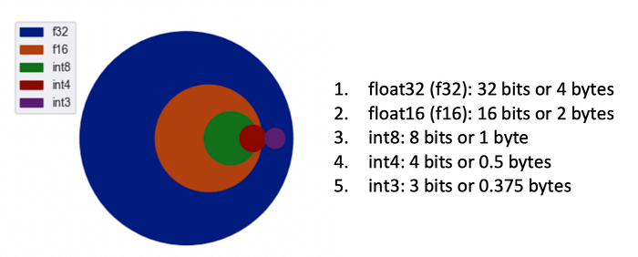
For geeks delving into the world of Large Language Models (LLMs) in generative AI, achieving rapid and precise results is of paramount importance. LLMs, notorious for their voracious appetite for resources such as GPUs, memory, and inference times, often pose a challenge for those lacking access to state-of-the-art hardware. Consequently, the tech-savvy community is actively exploring methodologies for executing these LLMs on more modest hardware setups, ensuring reduced memory usage, and facilitating high-quality outputs with minimal latency.
A typical LLM comprises a matrix of numerical values, commonly referred to as weights. One way to minimize memory consumption is to convert these weights into more efficient data types through a process known as quantization. By embracing this technique, even the most resource-intensive LLMs can be adapted for execution on less powerful hardware, without compromising the speed or accuracy of the generated responses.

As we saw above float 32(high-precision) occupies 4 bytes of memory. If we convert that value to int 8 then the size occupied by it will be reduced to 1/4th. So if a 13B parametre LLM model is 26GB then its int 8 quantization will be 26/4 ~ 6GB which reduces drastically and can be executed without any resource-constricted devices (like multi GPUs). Here are some pros and cons of using quantization on LLMs —
Pros:
Using smaller precision representations require less memory, which simplifies the deployment of models on devices with limited resources.
On hardware with efficient integer operations, such as CPUs, GPUs, and TPUs, quantized models execute quickly.
On mobile devices and in data centers, lower-precision computations are more energy-efficient.
Cons:
Due to precision loss, quantization might diminish model accuracy and negatively affect task performance.
The process of quantization is intricate and lengthy, requiring additional training steps.
Quantization methods can be split into two main categories: during training and post-training. Quantization during training changes the models while they’re being trained or fine-tuned. Quantization happens usually lengthy process of retraining and/or fine-tuning models. This method uses an approximate differentiation technique to handle the rounding operation that also require more resources. On the other hand, post-training methods, or “one-shot” methods, are like a quick makeover for pre-trained models. They only need a few thousand data samples and a few hours of work.
Post-training approaches are super interesting for massive models because training or fine-tuning them can be really costly. In this case, we’re focusing on post-training methods since they’re a bit easier on the wallet and perfect for big models.

The process of conversion warrants a closer examination. As is commonly known, an LLM model essentially consists of a high-dimensional matrix populated with numerical values. For the sake of simplicity, let us consider a 3x3 matrix as illustrated above, containing floating-point 32-bit (f32) numbers. To transform this into an 8-bit integer (int8) matrix, we must first understand the range of values that int8 can accommodate, which lies between -127 and 127. Consequently, a scaling factor is required to facilitate the conversion from f32 to int8, as depicted in the accompanying image. Each value in the f32 matrix is then multiplied by the scaling factor and rounded to the nearest integer. For example, the value in position [1,1] undergoes the following transformation: 2.32 * 13.62 = 31.59, which approximates to 32. The result is a lower-precision matrix composed of int8 representations.
The explanation provided thus far offers a fundamental comprehension of the concept. However, one must acknowledge that f32 represents a higher precision, while int8 denotes a lower precision, which consequently impacts the model’s performance adversely. Therefore, it becomes imperative to refine the int8 matrix in a manner that minimizes this loss. Researchers have devised methodologies to achieve this through a series of steps, which we shall now examine in the context of GPTQ, specifically.
Layer-Wise Quantization — As a matrix contains certain dimension(layers), we have to make sure there is minimal loss in converting these values. Process starts by quantizing layer by layer with few data points by minimising the precision loss. This process occurs in multiple steps till the loss is minimised(sum of squared errors) in converting the whole matrix to a quantized version preserving the salient information of the full precision matrix.
Optimal Brain Quantization — OBQ handles each row independently, quantizing one weight at a time while always updating all not-yet-quantized weights, in order to compensate for the error incurred by quantizing a single weight. All these operations happens on matrix with quantised and non quantised values are stored in a new matrix called Hessian. Few more mathematical operations undergo on the Hessian matrix row wise minimising the overall loss on all the weights present in the matrix. OBQ quantizes weights in greedy order, i.e. it always picks the weight which currently incurs the least additional quantization error. But running this on Billions of parametres is extremely expensive as it goes row by row and attends to each weight for minimizing loss.
Method proposed in GPTQ:
In GPTQ we convert f16 to int4. As OBQ method quantizes rows of W independently, in a specific order defined by the corresponding errors, the new method is to quantize the weights of all rows in the same order, and show that this typically yields results with a final squared error that is similar to the original solutions. This makes the process faster because certain computations have to be done only once for each column, rather than once for each weight.
To understand it the intricate mathematical details please refer to their research paper — https://arxiv.org/pdf/2210.17323.pdf
To implement this in python, we have a library called AutoGPTQ which can convert LLMs to quantised version using huggingface transformers https://github.com/PanQiWei/AutoGPTQ
Huggingface provided this colab notebook to understand how GPTQ quantization happens and how to infer GPTQ models in HuggingFace
Hope this article has cleared some air in understanding GPTQ. Happy reading ;)
